VLOOKUP Function
VLOOKUP Function
What is VLOOKUP
The VLOOKUP function (short for Vertical LOOKUP) is a built-in Calc function that is designed to work with data that is organized into columns. For a specified value, the function finds (or looks up) the value in one column of data, and returns the corresponding value from another column. Once you understand how VLOOKUP works and how to use it you will be able to create more sophisticated spreadsheets and further automate your work.
VLOOKUP example
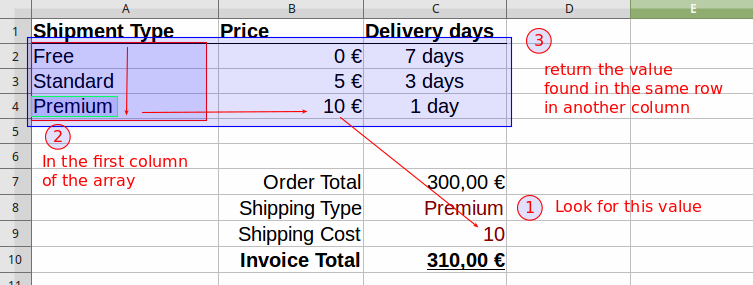
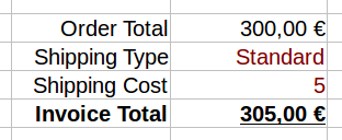
The VLOOKUP function is best explained using an example. In the spreadsheet below we calculate the Invoice Total as the sum of the Order Total plus the Shipping Cost.
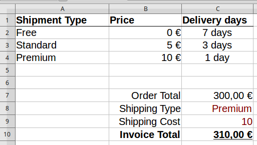
Instead of manually typing the Shipping Cost every time, VLOOKUP enables you to find the cost from the table above using the Shipping Type information ("Premium" in our example). You can probably already see in our example, at a glance, what is the cost of shipping, but on a more complex spreadsheet this information might be out of view, or even on another sheet. It is also shown by the example that with VLOOKUP we can refer to properties or values of a category simply by its name.
Using VLOOKUP
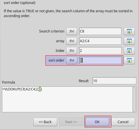
Lets insert the VLOOKUP formula into the Shipping Cost cell (C9). VLOOKUP has a lot of arguments therefore it is best to use the function wizard  . Select the cell C9 where the VLOOKUP function will be inserted. On the Function Wizard window select the Spreadsheet function category and choose the VLOOKUP function from the bottom of the list. Now you have to fill the four arguments that VLOOKUP requires.
-
Search criterion. This is the value that is searched for in the first column of the data table. In our example we are looking for the "shipping type" contained in cell C8.
-
Array. Now you must tell VLOOKUP the array where to look for the search criterion. In our example the array is the cell range A2:C4. VLOOKUP will search for the criterion in the first column of the array. One must ask why we give the array and not just the first column? The answer is because VLOOUKP needs the array not only to search but to return results from the other columns.
-
Index. The third argument is the column number from which the value will be returned. The first column has index 1, column 2, etc. In our example, we try to find the shipping cost contained in the second column.
-
Sort order. The last argument is optional but you are advised to use 0 or FALSE. When the sort order is 0 and a search term is not found, VLOOKUP returns an error message. If you skip this argument, the default value will be 1 or TRUE. In this case, VLOOKUP will always return the result of the last row even if the search does not match the term. This can easily lead to bugs in your spreadsheet if you do not know exactly how VLOOKUP works.
When you finish and click OK the formula result will be displayed in the cell with the Shipping Cost.
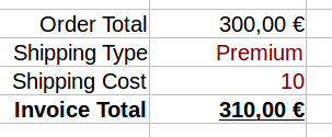
Now if you change the Shipping Type to "Standard" the Shipping Cost automatically calculates to the value of 5
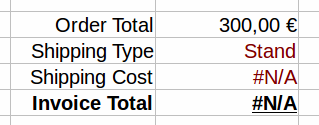
However if you insert a value that is not found on the array VLOOKUP will output an error. However, if you have assigned a sort order of 1 then the last ranked result will be returned.
How VLOOKUP works
Now that you have seen an example we can summarize how VLOOKUP function works.
-
Look for a value (for example "Premium") specified in the search criterion.
-
Define the a range that contains the column to look for and the columns to return results in the array argument. VLOOKUP will always search the first column in this range.
-
Now return the value that is in the same row with the matching result and in the column specified by the column index.
-
Use sort order 0, except when you have very large arrays and the first column is sorted.