Pivot Tables
Pivot Tables
Pivot Tables are one of the most powerful and useful tools in Calc. With this tool you can combine, compare, and analyzing large amounts of data easily. Using Pivot Tables, you can view different summaries of the source data, display the details of areas of interest, and create reports.
Why use Pivot Tables
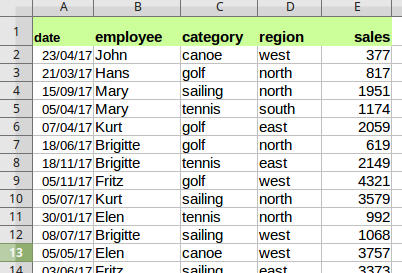
To better understand pivot tables let's examine an example. The spreadsheet below records sales from a company. To answer the question what is the amount sold by each salesperson it could be time consuming and difficult because each salesperson appears on multiple rows. We could use the Subtotal command to find the total for each salesperson, but we would still have a lot of data to work with.
Creating Pivot Table
Pivot table can created on data that have the table format which means no empty columns or rows and the first row contains the column names.
To create a Pivot Table:
Select only one cell from your data.
Choose the Insert Pivot Table command from the main menu or click the ![]() from the Standard toolbar.
from the Standard toolbar.
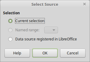
Calc automatically selects all the cells and opens the Select Source dialog. Click OK to continue
In the Pivot Table Layout Dialog you set up the pivot table. In general you drag fields from the Available Fields pane to the other white areas.
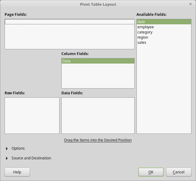
Drag the employee field to the Row fields are and the sales field to the Data Fields area and click OK.

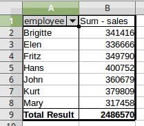
The pivot table is created in a new sheet. Now we get a summary of the sum of sales for each employee.
Pivot Table Layout
The layout of the pivot table is divided into 4 parts: Rows, Columns, Data and Page. If you understand the layout you will be able to create more complex pivot tables and extract important information from your data.
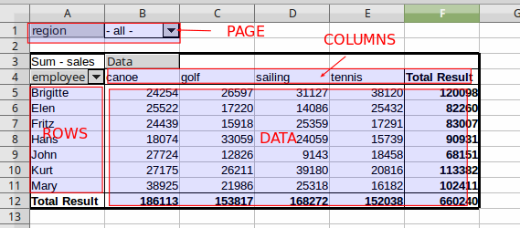
The Rows Area
When you drag a field into the Rows area of the pivot table, all the unique values in that field will be displayed in the first column of the pivot. The pivot table removes all the duplicates in the field (column of source data) and only displays the unique values. In the example we used the employee field for the Row area.
The Data Area
The Values area displays the data (values) that we want to summarize in our pivot table report. When you drag a field into the Values area, the pivot table will automatically sum or count the data in that field. If the data in the field contains numbers, then the sum will be calculated. If the data contains text or blanks, then the count will be calculated.
The Columns Area
The Columns area works just like the Rows area. It lists the unique values of a field in the pivot table. The only difference is that it lists the values across the top row of the pivot table. In the example above we used the category field in the Columns Area.
Page Area
Fields that are placed into the Page Fields area appear in the result above as a drop down list. The summary in your result takes only that part of your base data into account that you have selected. In the example above we used the region field in the Page Fields Area.
The best way to understand the pivot table layout and how to create pivot tables in general is to practice with various pivot table configurations and see the results
Edit a pivot Table
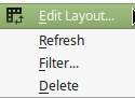
The real value of Pivot Tables is that they can quickly pivot (or reorganize) your data, allowing you to examine them in multiple ways. Pivoting data can help you answer different questions and discover new trends and patterns.To edit a pivot table layout, right click anywhere inside the Pivot Table and select Edit Layout from the context menu.
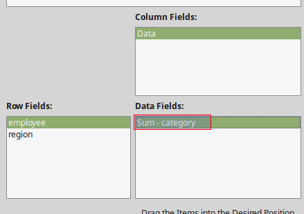
The Pivot Table Layout dialog window opens and allows you to delete, add or reorder fields in the layout.
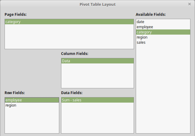
In our initial example we add the region fields to the Row area and the category fields to the Page area.

Updating the Pivot Table
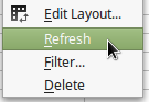
A Pivot Table will not update automatically if you change any of the data in your source sheet. To update, right click anywhere inside the Pivot Table and select Refresh from the context menu.
Data Fields calculation
By default numerical fields that are placed in the Data area are summarized with the SUM function. For text fields the default calculation is the COUNT function. This is why it's important to make sure you don't mix data types for value fields. You can change the calculation of a Data field in the Pivot Table Layout window.
To change the calculation double click on the field in the Data area.
In the Data Field pop up window select the function and click OK
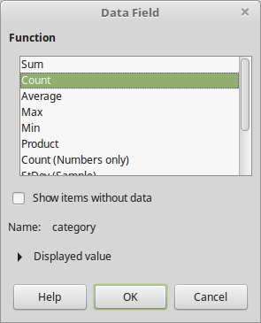
The following pivot table example uses the COUNT function for the category field

Delete a Pivot Table
To delete a pivot table, right click anywhere inside the Pivot Table and select Delete from the context menu.