Conditional Formatting

Conditional formatting provides another way to visualize data inside a spreadsheet. Using this tool you can automatically apply formatting such as colors, icons, and data bars, to a range of cells based on a condition or cell value.

It is recommended not to overuse conditional formatting as this could have the opposite results and make your spreadsheet look confusing.

Calc provides the following conditional formating types:

• Condition
• Color Scale
• Data Bar
• Icon Set

Setting up conditional formating

To set up conditional formating use one of the conditional formatting buttons in the Formating Toolbar.

In general to setup conditional formating

1. Select the range of cells that you want to format
2. Click one of the formating types
3. On the Conditional Formating window set one or more conditions

Applying Color Scale

Use Color scale to set the background color of cells depending on the value of the data in a spreadsheet cell. Color scale can only be used when All Cells has been selected for the condition. You can use either two or three colors for your color scale. Click on the Color Scale button to open the Conditional Formatting window. The value and the type of the scale (percentile, percentage, maximum, minimum) determines the coloring of the cells.

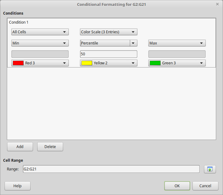
The results of color scale formatting are shown below. In our example, the closer the cell values approach to 50% of the age distribution become yellow. The upper and lower bounds of the distribution become green and red respectively.

Applying Data Bar

Data bars provide a graphical representation of data in your spreadsheet. The graphical representation is based on the values of data in a selected range. Data bars can only be used when All Cells has been selected for the condition. Use the  Data Bar button to open the Conditional Formatting window.

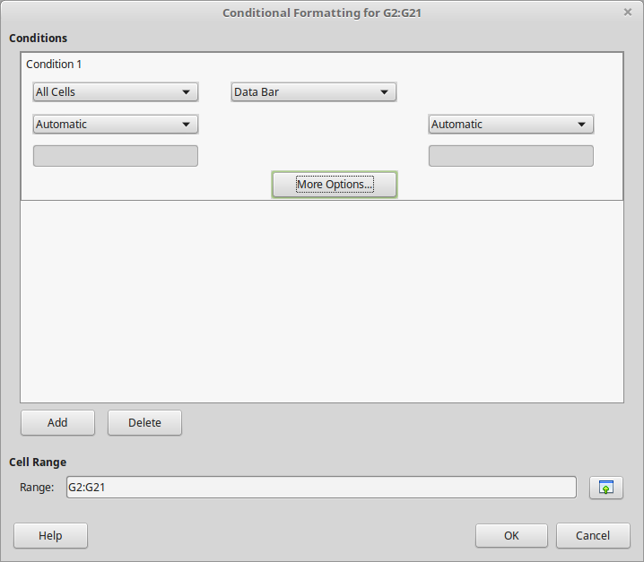
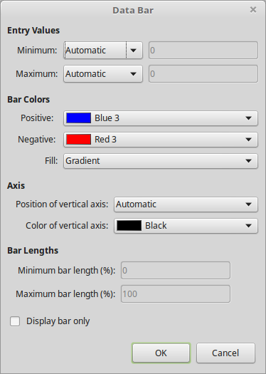
Click on More Options in the Conditional Formatting dialog to define how your data bars will look.

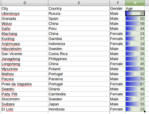
The data bar formating results are shown below. For each cell there is a small bar chart with a width depending on its value.

Applying Icon Set

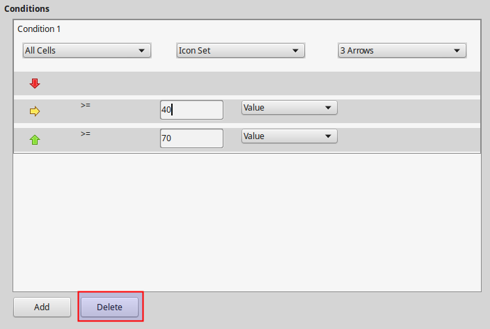
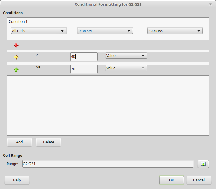
Icon sets display an icon next to your data in each selected cell to give a visual representation of where the cell data falls within the defined range that you set. The icons sets available are colored arrows, gray arrows, colored flags, colored signs, symbols, bar ratings and quarters. Icon sets can only be accessed when the Conditional Formatting dialog has been opened and All Cells has been selected for the condition. Use the Icon Set button to open the Conditional Formatting window. In our example, we fill in the two values that will define the three data ranges and their respective icons.

The results of Icon Set formating are shown below.

Applying Condition

With Condition you can apply a certain style to the data according to a condition you set. You can use the spreadsheet's predefined styles or create your own formating style before using this method. Use the  Condition button to open the Conditional Formatting window. In the following example we set a rule to apply the Result style to all cells with a value greater than 30.

The results of Condition are shown below.

Edit and Remove conditional formating

To Edit a conditional formating previously applied, select the cells, click on the used conditional formatting button and edit the condition parameters. You can also add condition using the Add Button. To remove a condition click the Delete button.