Sort, Filter and Format data

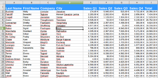
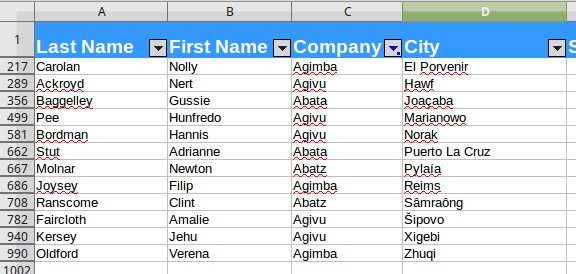
In this exercise you are given a spreadsheet with quarterly sales data. After you add a column to calculate the total you must format and filter the table. The end result is shown in the image below.

Instructions

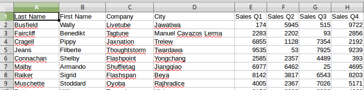
1. Open the file calc-filter-conditional-formating-exercise-start.ods. You will work on this document. The spreadsheet contains 1000 records of sales data.

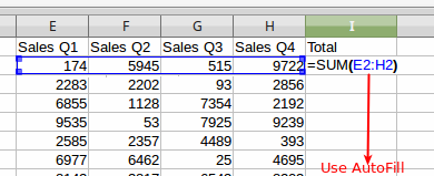
2. Create a column with the Total sales. Use the SUM function to add the cell range E2: H2 that contains the sales for each quarter. Then use autofill to fill the total to the remaining rows

3. Format the header. Increase font size, change background and/or font color. Format the numbers as currency.

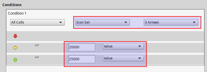
4. Apply conditional formating the the Total sales. Select the cell range I2:I1001 and apply Icon Set with the following values:

5. Apply automatic filter to the data. Select the first row and click the AutoFilter button.

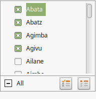
6. Filter the data by Company Name. Select only the first four companies:

7.  Sort the data by City name in ascending order

8. Save your file and submit.